Bulk RNA-seq PCA

workflowr

• Summary
• Checks
• Past versions

Last updated: 2021-08-16

Checks: 7 0

Knit directory: Turati_NatCancer_2021/

This reproducible R Markdown analysis was created with workflowr (version 1.6.2). The Checks tab describes the reproducibility checks that were applied when the results were created. The Past versions tab lists the development history.

---

R Markdown file: up-to-date

Great! Since the R Markdown file has been committed to the Git repository, you know the exact version of the code that produced these results.

Environment: empty

Great job! The global environment was empty. Objects defined in the global environment can affect the analysis in your R Markdown file in unknown ways. For reproduciblity it’s best to always run the code in an empty environment.

Seed: set.seed(20200627)

The command set.seed(20200627) was run prior to running the code in the R Markdown file. Setting a seed ensures that any results that rely on randomness, e.g. subsampling or permutations, are reproducible.

Session information: recorded

Great job! Recording the operating system, R version, and package versions is critical for reproducibility.

Cache: none

Nice! There were no cached chunks for this analysis, so you can be confident that you successfully produced the results during this run.

File paths: relative

Great job! Using relative paths to the files within your workflowr project makes it easier to run your code on other machines.

Repository version: 9254340

Great! You are using Git for version control. Tracking code development and connecting the code version to the results is critical for reproducibility.

The results in this page were generated with repository version 9254340. See the Past versions tab to see a history of the changes made to the R Markdown and HTML files.

Note that you need to be careful to ensure that all relevant files for the analysis have been committed to Git prior to generating the results (you can use wflow_publish or wflow_git_commit). workflowr only checks the R Markdown file, but you know if there are other scripts or data files that it depends on. Below is the status of the Git repository when the results were generated:

Ignored files:
    Ignored:    .Rhistory
    Ignored:    .Rproj.user/
    Ignored:    bulkRNA/
    Ignored:    data/bulk4_counts.rda
    Ignored:    data/bulk4_dds.rda
    Ignored:    data/paper_palette.rda
    Ignored:    data/signatures.rda
    Ignored:    output/deseq2-mini_bulk4_dds.3pts-Treated-vs-Untreated.rds
    Ignored:    output/deseq2-mini_bulk4_dds.pt1-Treated-vs-Untreated.rds
    Ignored:    output/deseq2-mini_bulk4_dds.pt12-Treated-vs-Untreated.rds
    Ignored:    output/deseq2-mini_bulk4_dds.pt13-Treated-vs-Untreated.rds
    Ignored:    output/deseq2-mini_bulk4_dds.pt2-Acutely treated-vs-Chronically treated.rds
    Ignored:    output/deseq2-mini_bulk4_dds.pt2-Acutely treated-vs-Never treated.rds
    Ignored:    output/deseq2-mini_bulk4_dds.pt2-Chronically treated-vs-Never treated.rds
    Ignored:    output/deseq2-mini_bulk4_dds.pt2-Relapse-vs-Never treated.rds
    Ignored:    output/deseq2-mini_bulk4_dds.pt2-Treatment withdrawn-vs-Never treated.rds
    Ignored:    output/fgsea_results.RDS
    Ignored:    output/figures/ExtFig5a_pca_3patients.pdf
    Ignored:    output/figures/ExtFig5b_pca_treatment_response.pdf
    Ignored:    output/figures/Fig5C_fgsea_selected_signatures.pdf
    Ignored:    output/figures/ItemS2.pdf
    Ignored:    output/tables/ExtFig5a_bulkRNAseq_data.xlsx
    Ignored:    output/tables/ExtFig5b_bulkRNAseq_data.xlsx

Note that any generated files, e.g. HTML, png, CSS, etc., are not included in this status report because it is ok for generated content to have uncommitted changes.

---

These are the previous versions of the repository in which changes were made to the R Markdown (analysis/bulkRNA-pca.Rmd) and HTML (docs/bulkRNA-pca.html) files. If you’ve configured a remote Git repository (see ?wflow_git_remote), click on the hyperlinks in the table below to view the files as they were in that past version.

File	Version	Author	Date	Message
html	b6f5b35	Javier Herrero	2021-08-13	Build site.
html	537463a	Javier Herrero	2021-08-13	Update site
Rmd	146911e	Javier Herrero	2021-08-13	Adding Bulk RNAseq / PCA page
html	146911e	Javier Herrero	2021-08-13	Adding Bulk RNAseq / PCA page

---

Introduction

library(ggbiplot)
library(tidyverse)
library(DESeq2)
# knitr::opts_chunk$set(cache = T, autodep = T)

num_of_genes.pca <- 1000

In this document, we are looking at the main components separating the samples, using PCA as an analyisis tool. We will use the top 1000 most variable genes.

Please refer to the Data - Bulk RNAseq page for more info.

data("bulk4_dds")
data("paper_palette")

plot_PCAs_from_vst <- function(vst, num.genes = 1000) {
  gene_variance <- rowVars(assay(vst))

  # select the 1000 top genes by variance
  selected_genes <- order(gene_variance, decreasing=TRUE) %>% head(n = num.genes)
  
  # perform a PCA on the data in assay(x) for the selected genes
  pca <- prcomp(t(assay(vst)[selected_genes, ]))
  
  pca_perc_variance <- round(1000 * pca$sdev^2 / sum(pca$sdev^2)) / 10
  
  pcaData <- pca$x[, 1:2] %>%
    as.data.frame() %>%
    rownames_to_column(var = "sample") %>%
    left_join(colData(vst) %>% as_tibble(), by = c("sample"))
  
  range_x <- range(pcaData$PC1)
  range_y <- range(pcaData$PC2)
  
  if (length(unique(pcaData$patient)) > 1) {
    ell_patients_groups <- pcaData %>% group_by(patient, group) %>%
      dplyr::summarise(n = n()) %>% filter(n > 2)
    ell <- list()
    apply(ell_patients_groups, 1, function(x) {
      this_patient = x[1]
      this_group = x[2]
      data <- pcaData %>% filter(patient == this_patient & group == this_group)
      this_ell <- car::dataEllipse(x = data$PC1, y = data$PC2,
                                   levels = 0.68, segments = 100,
                                   draw = F)
      ell[[paste(this_patient, this_group)]] <<-
        tibble(patient = this_patient, group = this_group,
               x = this_ell[1:100, 1], y = this_ell[1:100, 2],
             xend = this_ell[c(2:100, 1), 1], yend = this_ell[c(2:100, 1), 2])
      
    })
    ell <- Reduce(rbind, ell)

    g2 <- ggplot(pcaData, aes(PC1, PC2))
    if (length(ell) > 0) {
      g2 <- g2 +
        geom_segment(data = ell,
                     aes(x=x, y=y, xend=xend, yend=yend,
                         group=group, col=group, linetype = patient))
    }
    g2 <- g2 +
      geom_point(aes(col = group, shape = patient), size = 3) +
      # ggrepel::geom_text_repel(aes(label = sample), size = 2) +
      xlab(paste0("PC1: ", pca_perc_variance[1],"% variance")) +
      ylab(paste0("PC2: ", pca_perc_variance[2],"% variance")) +
      scale_colour_manual(values = paper_palette) +
      scale_fill_manual(values = paper_palette) +
      coord_fixed(ratio = diff(range_x) / diff(range_y)) +
      theme_bw(base_line_size = 0)
    g1 <- g2 +
      ggrepel::geom_text_repel(aes(label = sample), size = 2)

    ell_groups <- pcaData %>% group_by(group) %>%
      dplyr::summarise(n = n()) %>% filter(n > 2) %>% pull(group)
    ell <- lapply(ell_groups, function(name) {
      data <- pcaData %>% filter(group == name)
      car::dataEllipse(x = data$PC1, y = data$PC2,
                       levels = 0.68, segments = 100,
                       draw = F)
    })
    names(ell) <- ell_groups
    ell <- lapply(names(ell), function(name) {
      tibble(group = name, x = ell[[name]][1:100, 1], y = ell[[name]][1:100, 2],
             xend = ell[[name]][c(2:100, 1), 1], yend = ell[[name]][c(2:100, 1), 2])
      })
    ell <- Reduce(rbind, ell)
    
    g3 <- ggplot(pcaData, aes(PC1, PC2))
    if (length(ell) > 0) {
      g3 <- g3 +
        geom_segment(data = ell,
                     aes(x = x, y = y, xend = xend, yend = yend,
                         group = group, col = group))
      
    }
    g3 <- g3 +
      stat_ellipse(aes(col = group), level = 0.68, type = "norm") +
      geom_point(aes(col = group, shape = patient), size = 3) +
      # ggrepel::geom_text_repel(aes(label = sample), size = 2) +
      xlab(paste0("PC1: ", pca_perc_variance[1],"% variance")) +
      ylab(paste0("PC2: ", pca_perc_variance[2],"% variance")) +
      scale_colour_manual(values = paper_palette) +
      scale_fill_manual(values = paper_palette) +
      coord_fixed(ratio = diff(range_x) / diff(range_y)) +
      theme_bw(base_line_size = 0)
    
    print(g1)
    print(g2)
    print(g3)
    
    return(invisible(list(pcaData, g1, g2, g3)))
    
  } else {
    ell_groups <- pcaData %>% group_by(group) %>%
      dplyr::summarise(n = n()) %>% filter(n > 2) %>% pull(group)
    ell <- lapply(ell_groups, function(name) {
      data <- pcaData %>% filter(group == name)
      car::dataEllipse(x = data$PC1, y = data$PC2,
                       levels = 0.68, segments = 100,
                       draw = F)
    })
    names(ell) <- ell_groups
    ell <- lapply(names(ell), function(name) {
      tibble(group = name, x = ell[[name]][1:100, 1], y = ell[[name]][1:100, 2],
             xend = ell[[name]][c(2:100, 1), 1], yend = ell[[name]][c(2:100, 1), 2])
      })
    ell <- Reduce(rbind, ell)

    g2 <- ggplot(pcaData, aes(PC1, PC2))
    if (length(ell) > 0) {
      g2 <- g2 +
        geom_segment(data = ell,
                     aes(x = x, y = y, xend = xend, yend = yend,
                         group = group, col = group))
      
    }
    g2 <- g2 +
      geom_point(aes(fill = group), shape = 21, color = "black", size = 3) +
      xlab(paste0("PC1: ", pca_perc_variance[1],"% variance")) +
      ylab(paste0("PC2: ", pca_perc_variance[2],"% variance")) +
      scale_colour_manual(values = paper_palette) +
      scale_fill_manual(values = paper_palette) +
      coord_fixed(ratio = diff(range_x) / diff(range_y)) +
      theme_bw(base_line_size = 0)
    g1 <- g2 +
      ggrepel::geom_text_repel(aes(label = sample), size = 2)

    print(g1)
    print(g2)

    return(invisible(list(pcaData, g1, g2)))
  
  }
  
}

We transform the data all together with the VST transformation function. This essentially log-transforms the counts while taking into account the library size (see DESeq2 manual for more info).

bulk4_vst <- vst(bulk4_dds)

Treated vs untreated samples

All samples

This is the initial PCA, built from the bulk4_dds data set, using VST-transformed counts.

this_bulk_vst <- bulk4_vst[, colData(bulk4_dds)$patient %in% c("PT1", "PT12", "PT13")]
this_bulk_vst$patient <- factor(c("Pt1", "Pt2", "Pt12", "Pt13")[as.numeric(this_bulk_vst$patient)])
plots <- plot_PCAs_from_vst(this_bulk_vst)

`summarise()` regrouping output by 'patient' (override with `.groups` argument)

`summarise()` ungrouping output (override with `.groups` argument)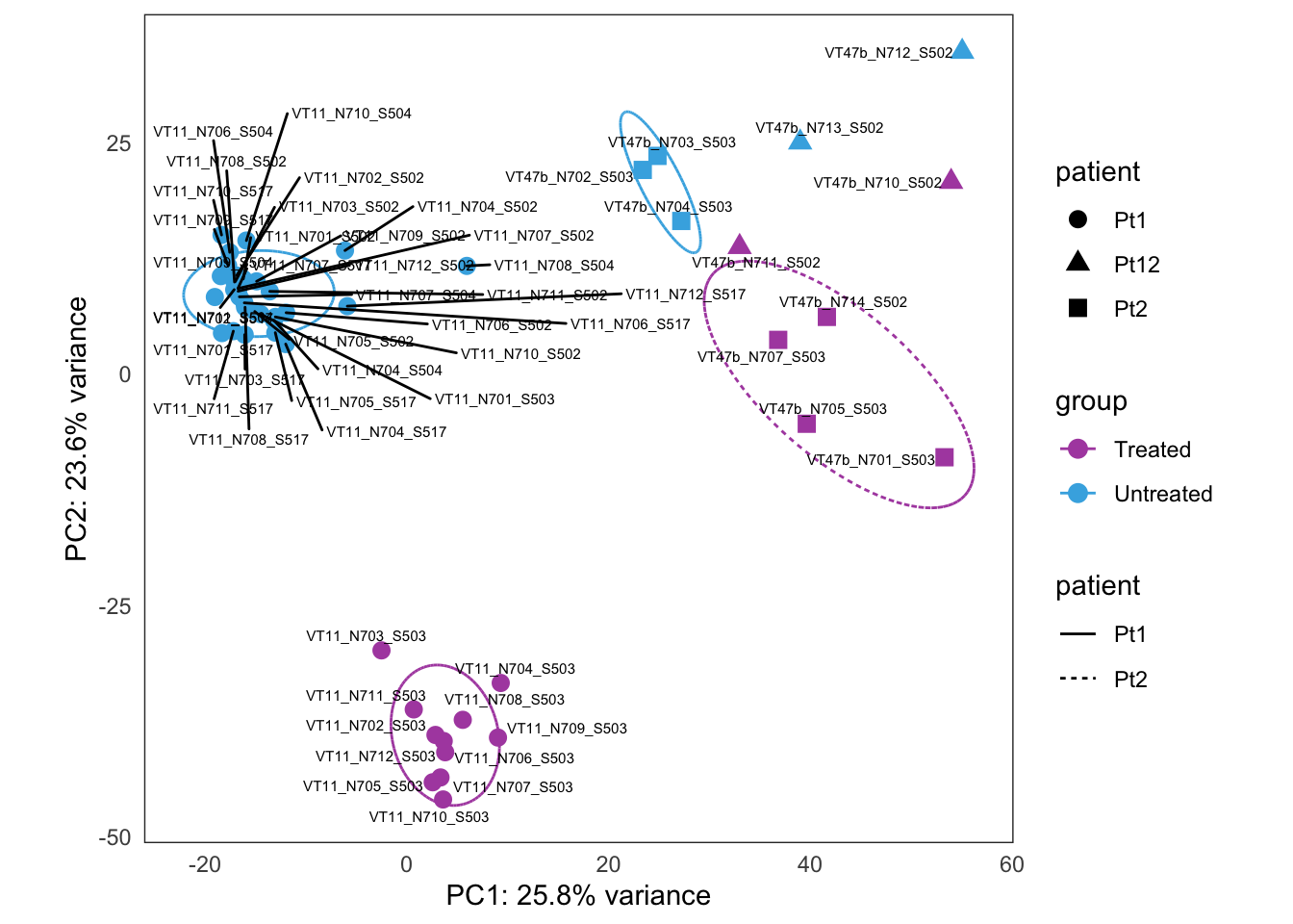

Past versions of treated_vs_untreated-1.png

Version	Author	Date
537463a	Javier Herrero	2021-08-13
146911e	Javier Herrero	2021-08-13

Past versions of treated_vs_untreated-2.png

Version	Author	Date
146911e	Javier Herrero	2021-08-13

Past versions of treated_vs_untreated-3.png

Version	Author	Date
146911e	Javier Herrero	2021-08-13

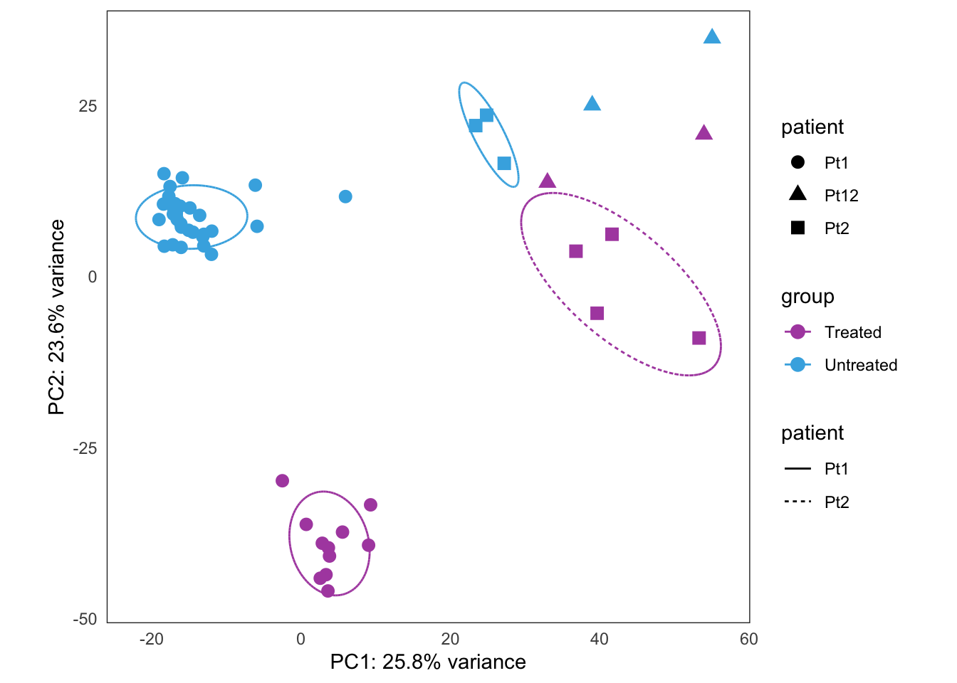
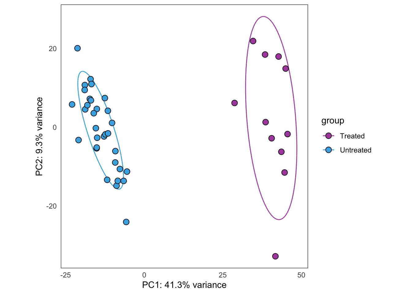
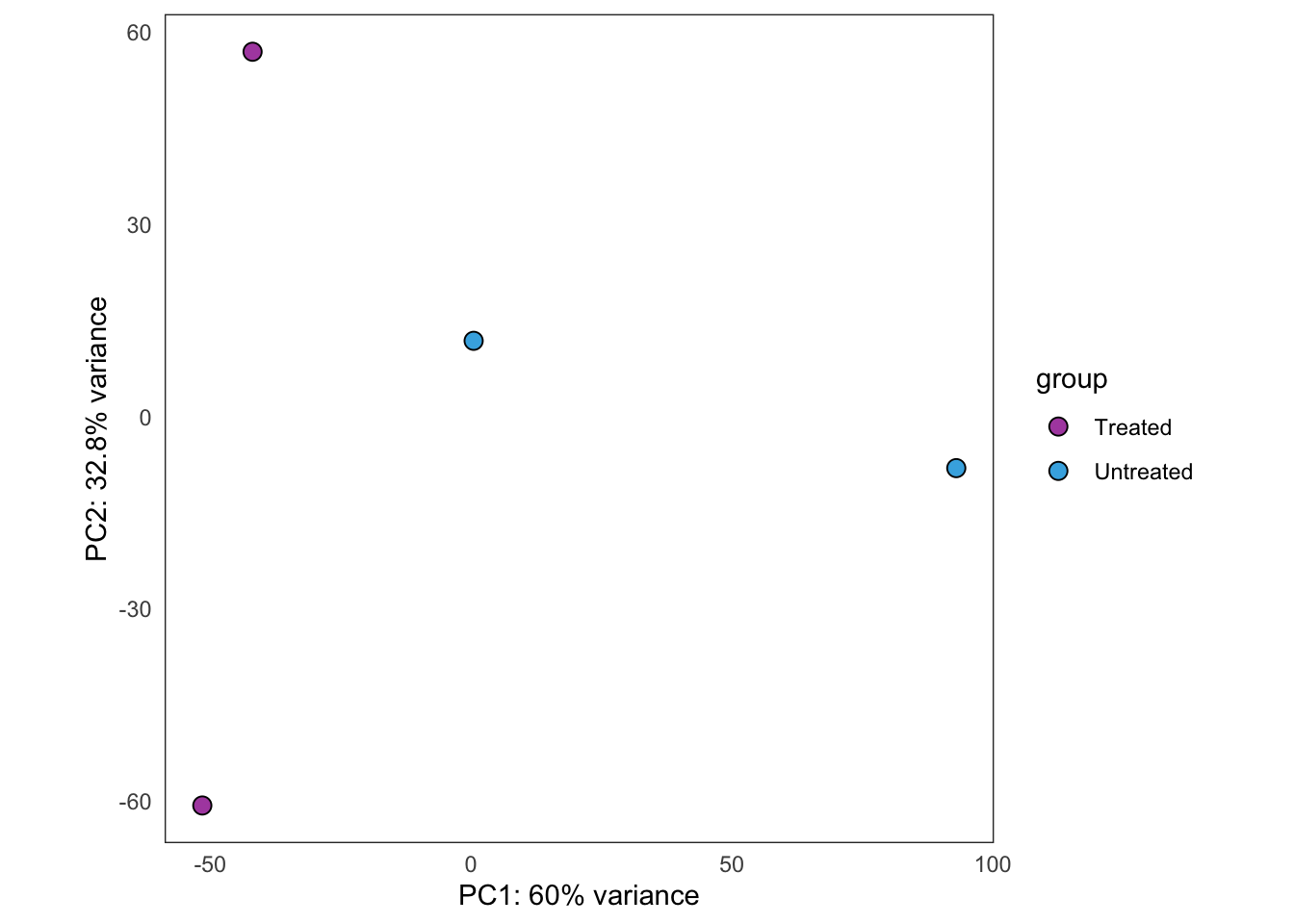
Extended Figure 5a

The next chunk of code save the ExtFig5a figure and associated data into the output folder

plots[[4]] +
  coord_cartesian() +
  guides(color = "none") +
  guides(shape = guide_legend(title = "Patient")) +
  theme(legend.position = "top")

Coordinate system already present. Adding new coordinate system, which will replace the existing one.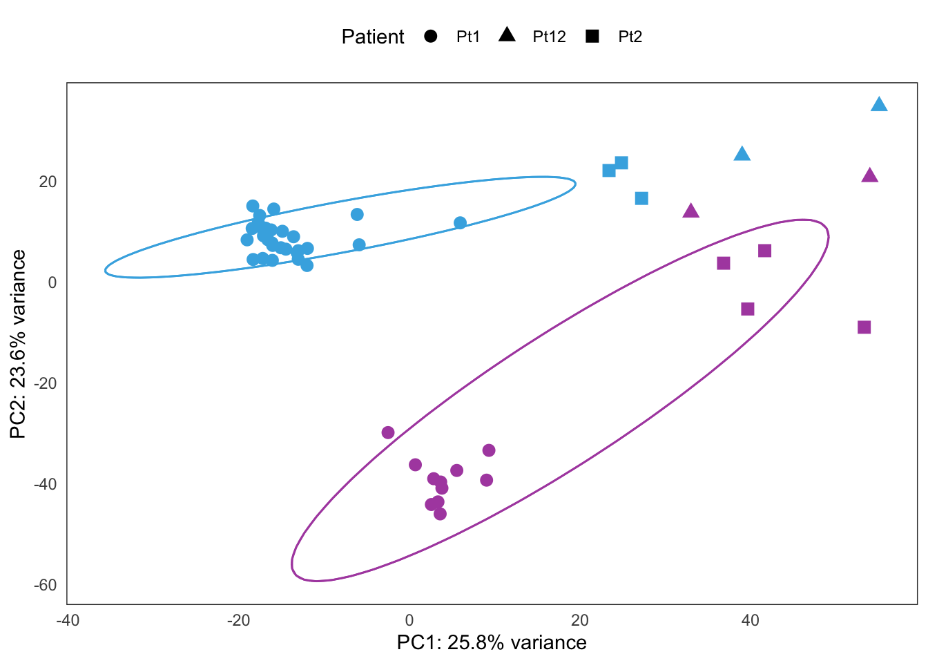

Past versions of save_extfig_5a-1.png

Version	Author	Date
146911e	Javier Herrero	2021-08-13

ggsave("output/figures/ExtFig5a_pca_3patients.pdf",
       device = "pdf", width = 5, height = 4, scale = 0.8)

excel_data <- plots[[1]]

wb <- openxlsx::createWorkbook()
ws <- openxlsx::addWorksheet(wb, "ExtFig5a PCA bulk RNAseq")

openxlsx::writeDataTable(wb, sheet = ws, x = excel_data,
               rowNames = F, tableStyle = "none", withFilter = F)
openxlsx::setColWidths(wb, ws, cols = 1:ncol(excel_data), widths = "auto")
openxlsx::addStyle(wb, ws, rows = 1, cols = 1:ncol(excel_data),
                   style = openxlsx::createStyle(textDecoration = "bold"))
openxlsx::addStyle(wb, ws, rows = 1:nrow(excel_data) + 1, cols = 1,
                   style = openxlsx::createStyle(textDecoration = "bold"))

openxlsx::saveWorkbook(wb, "output/tables/ExtFig5a_bulkRNAseq_data.xlsx", overwrite = TRUE)

PT1 only

Same as above, but using samples from PT1 only.

this_bulk_vst <- bulk4_vst[, colData(bulk4_dds)$patient %in% c("PT1")]
plot_PCAs_from_vst(this_bulk_vst)

`summarise()` ungrouping output (override with `.groups` argument)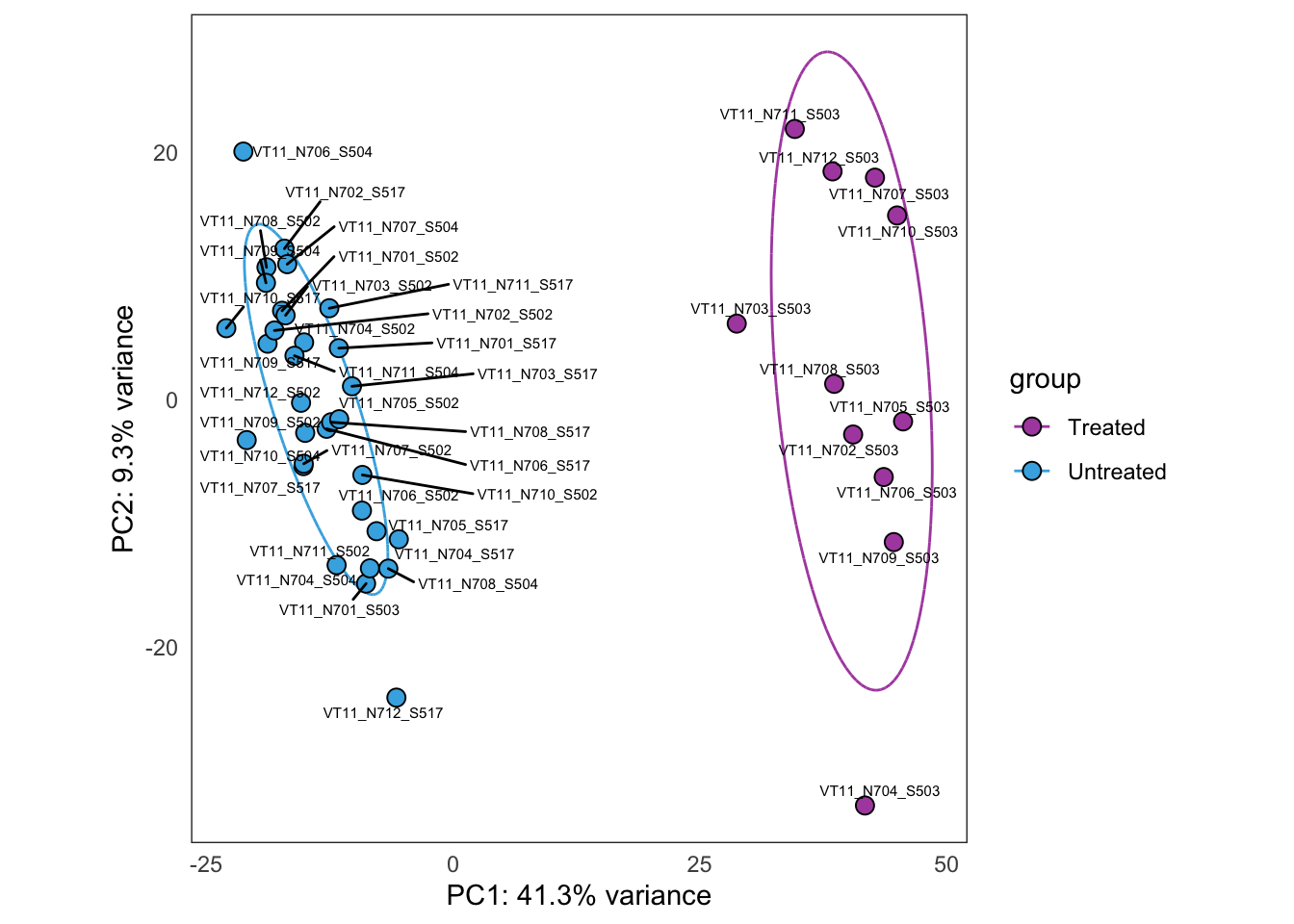

Past versions of treated_vs_untreated.pt1-1.png

Version	Author	Date
537463a	Javier Herrero	2021-08-13
146911e	Javier Herrero	2021-08-13

Past versions of treated_vs_untreated.pt1-2.png

Version	Author	Date
146911e	Javier Herrero	2021-08-13

PT12 only

Same as above, but using samples from PT12 only.

this_bulk_vst <- bulk4_vst[, colData(bulk4_dds)$patient %in% c("PT12")]
plot_PCAs_from_vst(this_bulk_vst)

`summarise()` ungrouping output (override with `.groups` argument)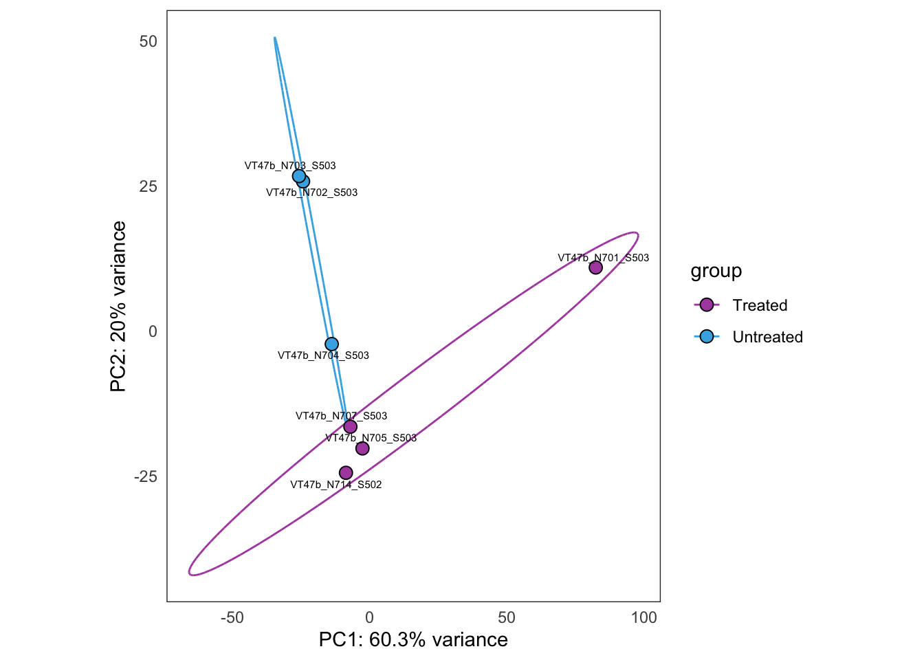

Past versions of treated_vs_untreated.pt12-1.png

Version	Author	Date
537463a	Javier Herrero	2021-08-13
146911e	Javier Herrero	2021-08-13

Past versions of treated_vs_untreated.pt12-2.png

Version	Author	Date
146911e	Javier Herrero	2021-08-13

PT13 only

Same as above, but using samples from PT13 only.

this_bulk_vst <- bulk4_vst[, colData(bulk4_dds)$patient %in% c("PT13")]
plot_PCAs_from_vst(this_bulk_vst)

`summarise()` ungrouping output (override with `.groups` argument)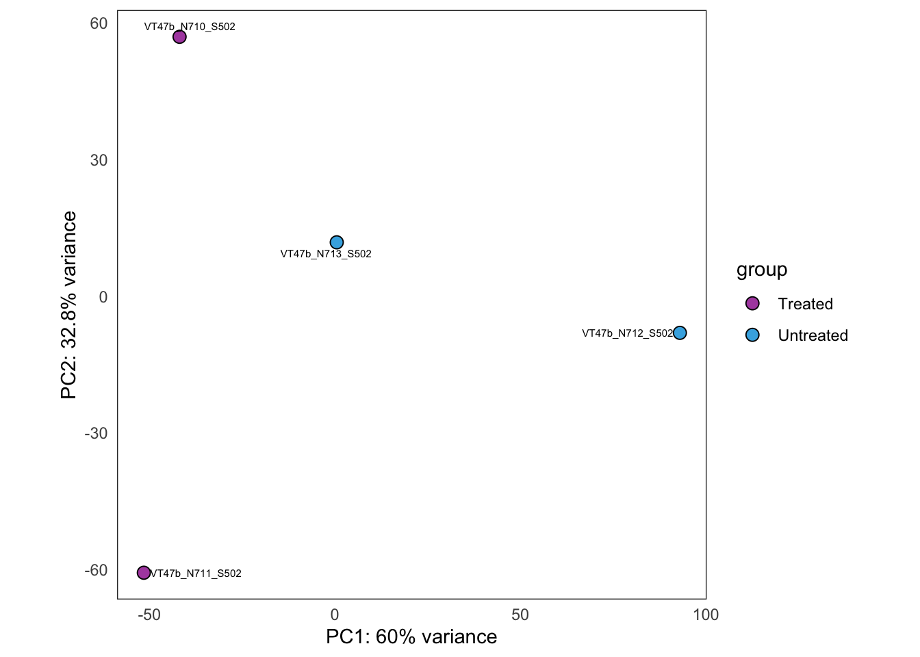

Past versions of treated_vs_untreated.pt13-1.png

Version	Author	Date
537463a	Javier Herrero	2021-08-13
146911e	Javier Herrero	2021-08-13

Past versions of treated_vs_untreated.pt13-2.png

Version	Author	Date
146911e	Javier Herrero	2021-08-13

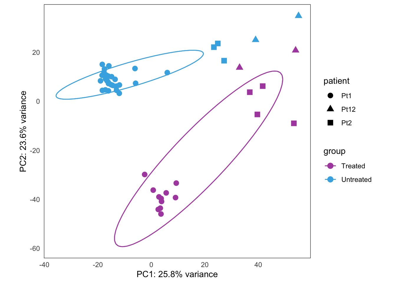
Treatment response experiment

This is the initial PCA, built from the bulk4_dds data set, using VST-transformed counts. The data correspond to PT2, where we have five types of samples:

• untreated
• treatment withdrawn
• chronically treated
• acutely treated
• relapse (let to relapse)

this_bulk_vst <- bulk4_vst[, colData(bulk4_dds)$patient %in% c("PT2")]
hack_bulk_vst <- this_bulk_vst
hack_bulk_vst$patient <- hack_bulk_vst$tissue
plots <- plot_PCAs_from_vst(hack_bulk_vst)

`summarise()` regrouping output by 'patient' (override with `.groups` argument)

`summarise()` ungrouping output (override with `.groups` argument)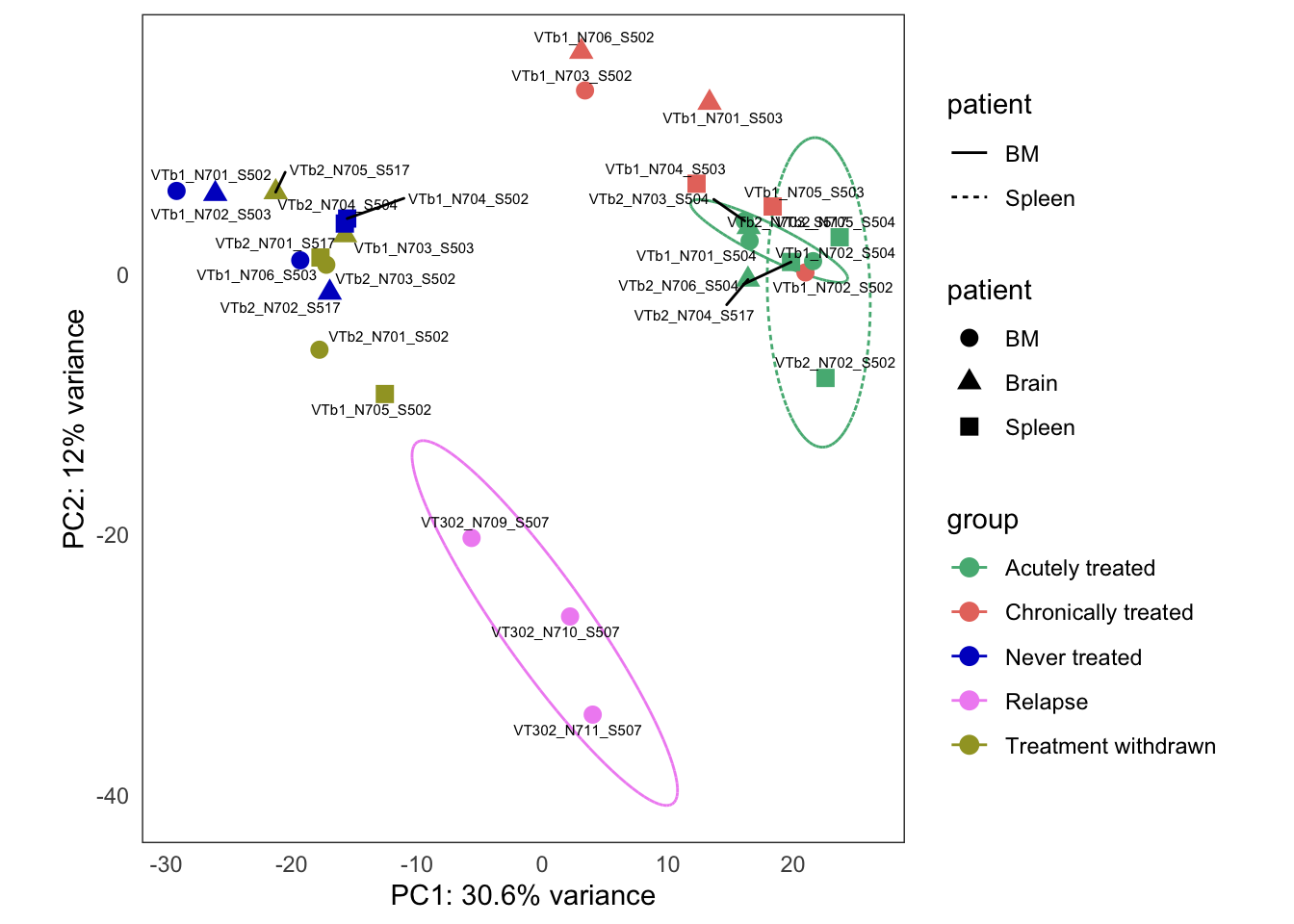

Past versions of treatment_response-1.png

Version	Author	Date
537463a	Javier Herrero	2021-08-13
146911e	Javier Herrero	2021-08-13

Past versions of treatment_response-2.png

Version	Author	Date
146911e	Javier Herrero	2021-08-13

Too few points to calculate an ellipse

Warning: Removed 1 row(s) containing missing values (geom_path).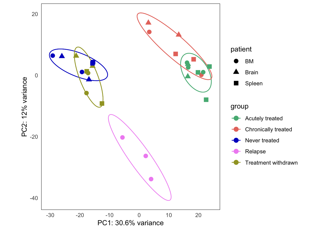

Past versions of treatment_response-3.png

Version	Author	Date
146911e	Javier Herrero	2021-08-13

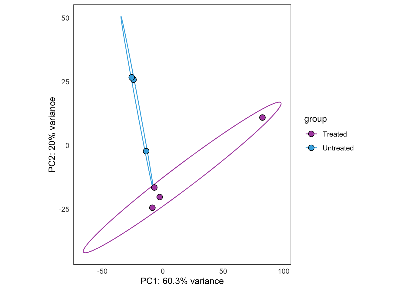
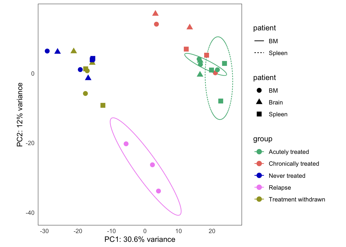
Extended Figure 5b

The next chunk of code save the ExtFig5b figure and associated data into the output folder

plots[[4]] +
  coord_cartesian() +
  guides(color = "none") +
  guides(fill = "none") +
  guides(shape = guide_legend(title = "Tissue")) +
  theme(legend.position = "top")

Coordinate system already present. Adding new coordinate system, which will replace the existing one.

Too few points to calculate an ellipse

Warning: Removed 1 row(s) containing missing values (geom_path).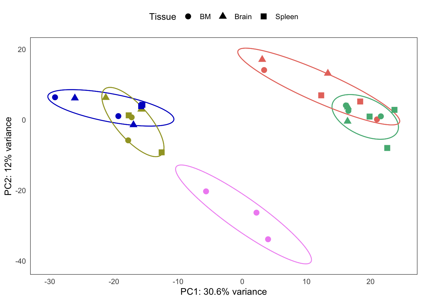

Past versions of save_extfig_5b-1.png

Version	Author	Date
146911e	Javier Herrero	2021-08-13

ggsave("output/figures/ExtFig5b_pca_treatment_response.pdf",
       device = "pdf", width = 6, height = 4, scale = 0.8)

Too few points to calculate an ellipse

Warning: Removed 1 row(s) containing missing values (geom_path).

excel_data <- plots[[1]]

wb <- openxlsx::createWorkbook()
ws <- openxlsx::addWorksheet(wb, "ExtFig5b PCA bulk RNAseq")

openxlsx::writeDataTable(wb, sheet = ws, x = excel_data,
               rowNames = F, tableStyle = "none", withFilter = F)
openxlsx::setColWidths(wb, ws, cols = 1:ncol(excel_data), widths = "auto")
openxlsx::addStyle(wb, ws, rows = 1, cols = 1:ncol(excel_data),
                   style = openxlsx::createStyle(textDecoration = "bold"))
openxlsx::addStyle(wb, ws, rows = 1:nrow(excel_data) + 1, cols = 1,
                   style = openxlsx::createStyle(textDecoration = "bold"))

openxlsx::saveWorkbook(wb, "output/tables/ExtFig5b_bulkRNAseq_data.xlsx", overwrite = TRUE)

Session information

sessionInfo()

R version 3.6.3 (2020-02-29)
Platform: x86_64-apple-darwin15.6.0 (64-bit)
Running under: macOS Catalina 10.15.7

Matrix products: default
BLAS:   /Library/Frameworks/R.framework/Versions/3.6/Resources/lib/libRblas.0.dylib
LAPACK: /Library/Frameworks/R.framework/Versions/3.6/Resources/lib/libRlapack.dylib

locale:
[1] en_GB.UTF-8/en_GB.UTF-8/en_GB.UTF-8/C/en_GB.UTF-8/en_GB.UTF-8

attached base packages:
 [1] parallel  stats4    grid      stats     graphics  grDevices utils    
 [8] datasets  methods   base     

other attached packages:
 [1] DESeq2_1.26.0               SummarizedExperiment_1.16.1
 [3] DelayedArray_0.12.3         BiocParallel_1.20.1        
 [5] matrixStats_0.56.0          Biobase_2.46.0             
 [7] GenomicRanges_1.38.0        GenomeInfoDb_1.22.0        
 [9] IRanges_2.20.2              S4Vectors_0.24.4           
[11] BiocGenerics_0.32.0         forcats_0.5.0              
[13] stringr_1.4.0               dplyr_1.0.0                
[15] purrr_0.3.3                 readr_1.3.1                
[17] tidyr_1.0.2                 tibble_2.1.3               
[19] tidyverse_1.3.0             ggbiplot_0.55              
[21] scales_1.1.0                plyr_1.8.6                 
[23] ggplot2_3.3.1               workflowr_1.6.2            

loaded via a namespace (and not attached):
  [1] colorspace_1.4-1       ellipsis_0.3.0         rio_0.5.16            
  [4] rprojroot_1.3-2        htmlTable_1.13.3       XVector_0.26.0        
  [7] base64enc_0.1-3        fs_1.3.2               rstudioapi_0.11       
 [10] farver_2.0.3           ggrepel_0.8.2          bit64_0.9-7           
 [13] AnnotationDbi_1.48.0   lubridate_1.7.4        xml2_1.2.5            
 [16] splines_3.6.3          geneplotter_1.64.0     knitr_1.28            
 [19] Formula_1.2-3          jsonlite_1.6.1         broom_0.5.5           
 [22] annotate_1.64.0        cluster_2.1.0          dbplyr_1.4.2          
 [25] png_0.1-7              compiler_3.6.3         httr_1.4.1            
 [28] backports_1.1.5        assertthat_0.2.1       Matrix_1.2-18         
 [31] cli_3.0.0              later_1.0.0            acepack_1.4.1         
 [34] htmltools_0.5.1.1      tools_3.6.3            gtable_0.3.0          
 [37] glue_1.3.2             GenomeInfoDbData_1.2.2 Rcpp_1.0.4            
 [40] carData_3.0-3          cellranger_1.1.0       vctrs_0.3.0           
 [43] nlme_3.1-145           xfun_0.16              openxlsx_4.1.4        
 [46] rvest_0.3.5            lifecycle_0.2.0        XML_3.99-0.3          
 [49] zlibbioc_1.32.0        hms_0.5.3              promises_1.1.0        
 [52] RColorBrewer_1.1-2     curl_4.3               yaml_2.2.1            
 [55] memoise_1.1.0          gridExtra_2.3          rpart_4.1-15          
 [58] latticeExtra_0.6-29    stringi_1.4.6          RSQLite_2.2.0         
 [61] genefilter_1.68.0      checkmate_2.0.0        zip_2.2.0             
 [64] rlang_0.4.11           pkgconfig_2.0.3        bitops_1.0-6          
 [67] evaluate_0.14          lattice_0.20-40        labeling_0.3          
 [70] htmlwidgets_1.5.1      bit_1.1-15.2           tidyselect_1.1.0      
 [73] magrittr_1.5           R6_2.4.1               generics_0.0.2        
 [76] Hmisc_4.3-1            DBI_1.1.0              pillar_1.4.3          
 [79] haven_2.2.0            whisker_0.4            foreign_0.8-76        
 [82] withr_2.4.2            abind_1.4-5            survival_3.1-11       
 [85] RCurl_1.98-1.1         nnet_7.3-13            car_3.0-8             
 [88] modelr_0.1.6           crayon_1.3.4           rmarkdown_2.1         
 [91] jpeg_0.1-8.1           locfit_1.5-9.1         readxl_1.3.1          
 [94] data.table_1.12.8      blob_1.2.1             git2r_0.26.1          
 [97] reprex_0.3.0           digest_0.6.25          xtable_1.8-4          
[100] httpuv_1.5.2           munsell_0.5.0